A Taxonomy of Biases in Marketing Mix Model Effect Estimation – Part 5

One of the interesting things about Marketing Mix Models in real life is that many different academic backgrounds have contributed to the current state of the industry. The earliest MMMs were_likely_ built at major CPG companies by operations research specialists or statisticians, then a spate of econometricians carried the idea of regression models to estimate marketing impact into a cottage industry. In my opinion, MMM was mostly ignored by the “data science is the sexiest job of the 21st century” crew, but as causal inference has become a data science topic and open source MMM packages were released in ‘data science-y’ languages it seems like MMM is now being carried forward with a focus on machine learning and automation. 

I bring that up because this post focuses on a bias that was named by econometricians; specifically folks trying to build systems of equations on time series data, called Structural Equation Models.  

Our topic today is endogeneity.   

Endogeneity Defined  

We have endogeneity when some features in the model are correlated to the error term in the model.  

The practical definition might be: “If you attempt to correct for endogeneity and it changes your effect estimates noticeably, then you have an endogeneity problem.” I wish that was a joke, but the Hausman test literally compares an endogeneity corrected estimate with an uncorrected one and looks to see if the uncorrected estimate is inconsistent (in the technical meaning of not asymptotically approaching the same value as sample size increases), with the corrected one. 

But How Can This Happen in My Model? 

Every introductory article (e.g. the excellent Wikipedia article) groups endogeneity into three causes: an unobserved confounder, measurement error, and simultaneity bias. 

An unobserved confounder occurs when a variable is left out of the model that is correlated to both an independent variable in the model and to the dependent variable. That should sound familiar to you, as we covered omitted variable bias back in Part 1 and the mechanism of action is the same! 

Here’s a quick walk through to show why omitting a variable leads to a correlation to the error term. Let’s start by assuming the real relationship between y, x, and z is 

(1)

Let’s also assume that z and x are not independent . . . note that we don’t care in this case if there is a true relationship between them or if they just happen to be correlated, but I’ll stick with the ‘assignment’ operator as a definition, like so 

(2)

So if our model is being built without z because it’s not available to us, or because we don’t realize it has an effect on our outcome of interest, we get 

(3)

Which we might expand to 

(4)

Of course, since z is correlated to x, so is ergo the error of our reduced form model is no longer independent of x.  

The second reason for endogeneity, which I strongly suspect was seen as the primary issue in the fields where endogeneity research took hold, is measurement error. One of the pesky assumptions about linear regression models is that independent variables are known exactly. In applied linear regression courses it is typical for an optional chapter, near the end of the book, to cover Error in Both Variables Modeling; somewhere in the intro section for that chapter there is a note suggesting that as long as the independent variables’ errors are much smaller than the error in the dependent variable it is reasonable to ignore violations of this assumption and use regular OLS. 

But in macroeconomics and psychology it is pretty common to have a system of equations where each term might be the left-hand side for some equations and the right-hand side for others. It is an interesting exercise in cognitive dissonance to quantify error in a variable for the equations where it is the dependent variable and then turn around and ignore the error for equations where it is an independent variable. As a result, those fields have long paid attention to measurement error and its impact on effect estimation. 

The ‘proof’ that measurement error can lead to endogeneity is essentially the same as for the unobserved confounder (and, perhaps, measurement error is exactly the same as an unobserved confounder?): 

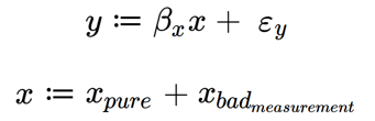
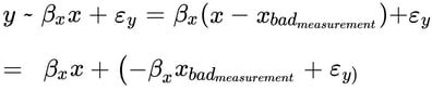
Where x and that grouped error term are not independent because they both depend on .

The 3rd source of endogeneity, like measurement error, arises in a system of equations, and especially in a system of equations involving time series data (exactly the data we use in marketing mix models!). It is typical to assume that a cause must precede its effect in philosophy and physical sciences.   

Unfortunately, in econometrics we often see the frequency of data sampling is low (monthly or quarterly) and so simultaneous effects are expected – basically for each egg laid we first have to have chicken to lay it, but if we are counting the annual chicken population and an annual number of eggs, we’d expect the two numbers to move together. In a system of equations describing the total egg industry using annual numbers, we might have: 

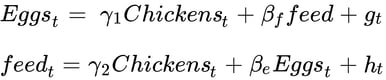
Where maybe feed depends on Eggs because heavy layers eat more? I don’t know; I’ve never raised chickens!  

But now you can see that any way we substitute from one of the equations into the other we are going to bring an error term along with us that will be associated with one of the predictors (and if it’s not clear, please actually read the Wikipedia article linked to earlier!)  

How Much Do I Need to Worry About This? 

As always, the answer is, “it depends!”  

I’ve created a quick example of the ‘unobserved confounder’ stripe. We can expect to have unobserved confounders of varying strengths in the real world, so I built 3 levels of confounding by varying the degree to which the unobserved variable influenced the error term in the model. 

The data ends up looking like this:

To show the impact of the varying levels of endogeneity, I’ve regressed the 3 rightmost columns on X, and recorded the estimated effect (i.e. the coefficient of X in those regressions): 

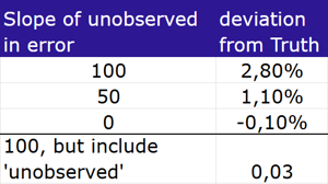
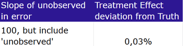
Unsurprisingly, ‘more endogeneity’ (i.e. a larger slope of the unobserved vs the error) results in a greater bias in our estimate.   

I also went ahead and regressed the Strong Endogeneity outcome on both X and the ‘Unobserved Driver’ (which has now magically become observed – this is why synthetic data is fun!) and get this: 

Demonstrating that specifying a model that perfectly matches the true data generating process leads to good outcomes. 

So do you have to worry about this?  Well, if my arbitrarily selected levels of endogeneity are representative of real life, I’d say no.  A 3% bias is small relative to the width of the confidence intervals we see in most MMMs . . . but of course we can’t be sure that our real endogeneity isn’t stronger than this example. 

Methodological Fixes 

Since in real life the unobserved confounders stay unobserved and the ‘degree of endogeneity’ is therefore incalculable, a lot of research has been done to find robust-to-endogeneity estimation methods. The approach with the most history is the use of instrumental variables in either a 2SLS or 3SLS regression. The difficulty with instrumental variables is that they need to be related to the endogenous variables in the model, but uncorrelated to the error . . . which is tricky when the endogenous variable is, by definition, correlated with the error. 

And so more recent approaches use latent instrumental variables or copula corrections instead. This isn’t a topic I have any particular expertise in, so I won’t rewrite the available information on these methods.  I will share that I’m currently working through real world examples using the 2sCOPE copula correction (here) and then intend to check into the multilevel GMM correction in the REndo package.  If you take either of these for a spin with real data and want to talk over the results, please reach out! 

Wrapping Up 

Endogeneity isn’t quite like the other named biases in the series in that there is very clearly a tradeoff between omitted variable bias and mediation bias and endogeneity doesn’t work that way.   

Marketing mix models almost always include some measurement error in the predictors (TV ratings points being the foremost example, but I’ve noticed impression and click counts for any given time period tend to change from one data pull to the next)  and some confounders will surely be unobserved (“uh, the team thinks that dip in sales lines up with the lawsuit press we had?”). But maybe there isn’t any reason to allow some of the sources of endogeneity to enter a model. I’m thinking especially of the simultaneous effects problem; if you are building a system of equations and it is possible to avoid specifying simultaneous effects, then avoidance is a great choice. 

Currently, the most common choice for MMM analysts is to know that endogeneity might be present (especially in the form of omitted variables or unobserved confounding) and hope that we can to ensure the impact is small by making careful choices of which variables to include in our model as ‘controls’ and then comparing our results to prior work. But this option might not be long for the world, as some literature reviews see endogeneity correction as increasingly common in marketing research.  I think it’s likely the practice of MMM will shift to match that interest. 

So perhaps you’ll join me in trying some of the approaches to endogeneity correction available to us? So far my selected test runs have not shown large shifts in estimates (relative to the typical uncertainty of estimates), but with the relatively weak assumptions of modern endogeneity corrections and the availability of open source software for estimation, it might soon be simpler to check if a correction is warranted than to argue that the effects are likely small. 

If you do decide to try a new estimation approach after reading this, drop me a line and tell me! I am very keen to see how this pans out for us marketing analysts.